
In-Space Electrical Propulsion
-
Introduction
Space Propulsion is a branch of engineering that is devoted to the study and characterization of propulsive systems that allow the operation of a spacecraft once they leave the Earth’s atmosphere. The defining characteristic of such systems –directly derived from their definition–, with respect to other forms of propulsion, lies in the fact that the environment on which they operate is a vacuum. As a consequence, they cannot take the advantage of any external medium in order to generate the forces needed to move the vehicle, as it is done, for instance, in the case of aircraft jet propulsion –in which this external medium is atmospheric air. This leads to the necessity of finding alternative means of generating those forces and designing devices that do not necessarily rely on any external supply for their operation. Amongst these relatively autonomous systems –a category that also includes not so conventional devices such as solar sails or tethers, to mention some– the most renowned one is the Rocket Engine.[1-2]
Rocket engines operate by discharging a mass of propellant into the surrounding space. The release of this mass of propellant –known as exhaust– entails a change in the momentum of the rocket system, opposite and equal in magnitude to the one conferred to the ejected particles in their expulsion, enabling the movement of the vehicle. This change in the momentum of the rocket, due to the ejection of the propellant, is known as Thrust (~T), and it is given –in the absence of pressure jumps at the exit section of the rocket’s nozzle– by:
(1) 
where the exhaust mass flux through a surface  is multiplied by the exit velocity to obtain the total momentum per unit time or thrust.
While the thrust of the engine is an important parameter to consider, in space propulsion, a second parameter known as the specific velocity represents the main indicator of the performance of a rocket engine. This specific velocity can be defined as the thrust divided by the ejected mass flow rate:
(2) 
This indicator of performance has been traditionally expressed in seconds and termed the specific impulse by dividing the magnitude of  by gravity:
(3) 
The reason for the Specific Impulse to be of such high importance can easily be explained using the modified Tsiolkovsky’s Generalized Rocket Equation momentum equation:
(4) 
where the gain in speed,  , needed for a long range mission is only given by the Specific Impulse and the initial and final masses. While higher Thrust allows you to gain speed faster, it is the Specific Impulse that will allow you to reach the speeds that are needed for prolonged missions.
The main research objective of the project undertaken is therefore to characterize a propulsive system that has the highest possible Specific Impulse using the smallest possible flow rate. Among the different sources of space propulsion such as nuclear or thermal, electric propulsion [3] has some of the largest advantages in terms of efficiency, simplicity, compactness, long life and accurate control. By the term electric propulsion, we refer to all those rocket engines where the source of energy is the electrical energy stored in batteries or other types of electric accumulators. That energy is then used to accelerate the propellant to very high velocities, in a process that can be carried out by different means such as ion thrusters, plasma hall thrusters, field emission thrusters and colloidal or pure ionic thrusters.
Among those of electrical propulsion, in this project we would like to study the propulsive characteristics of colloidal thrusters [4-5] and in particular a branch of such colloidal thrusters termed Pure Ionic thrusters [6-10] which can easily achieve Specific Impulses of over 10,000 and mission life in the order of decades. The liquids of choice that have sufficient electrical conductivity and high surface tension are termed Room Temperature Ionic Liquids [11-17] and correspond to imidazole type liquids. One of the interesting outcomes of the project is to test which of these liquids gives the highest performance factors and why.
Regarding its physical basis, colloidal propulsion represents a particular application of a more general problem in the field of electrohydrodynamics [18], known as nobel award winning technique called electrosprays [19-20], which leads to its alternative designation as electrospray-based space propulsion. The justification for colloidal or electrospray-based propulsion lies in the fact that, by means of electrospray atomization it is possible to generate –in a vacuum, as required in the space environment, and with relative ease– beams composed of particles with moderately high charge-to-mass ratios, which are subsequently accelerated to very high velocities by the same electric field involved in their formation.
In this project, the students will mimic space like conditions through the use of a vacuum chamber. A Time of Flight (ToF) will be used to study the exhaust speeds of the ion beam that will be collected and measured through an oscilloscope. The propulsive characteristics of different propellants will then be studied choosing the most appropriate.
-
Experimental Setup
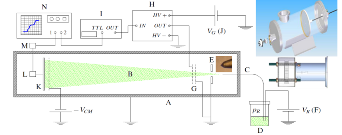
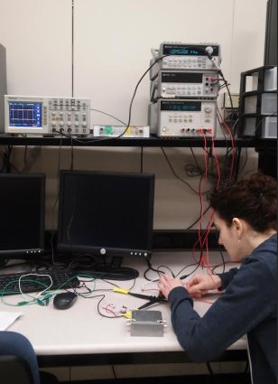
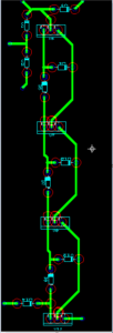
A experimental setup of the vacuum chamber is shown. Please refer to the text for the labeling of the different parts of the setup.
The experimental setup –sketched in Figure 1– consists, in short, of a vacuum chamber (A) inside of which a liquid is electrosprayed (B) from the tip of a capillary needle (C) and subject to Time of Flight measurements. The liquid is fed into the needle from a reservoir (D) set to a certain pressure PR with respect to the zero-pressure level inside the chamber (Poiselle’s Flow). To generate the electrospray, a high voltage level VR is applied to the liquid in the reservoir with respect to a grounded extractor (E), by means of a high voltage source (F) with currents in the range of nA. The Time of Flight measurements are performed by stopping and then releasing the beam with the aid of an electrostatic gate (G), subject to high voltage pulses generated by a high voltage switch (H). To generate these pulses, a low voltage pulse of the desired frequency is introduced in the switch from an output a wave generator (I) and then mixed with a high voltage level VG coming from an additional high voltage source (J). After being released, the beam is collected in a collector (K), where the received current signal is conditioned and amplified by means of an electrometer(L)-amplifier(M) group. This signal is then sent to the scope of an oscilloscope (N) triggered by a TTL-sync pulse coming from the wave generator, so that its zero-time reference is synchronized with the pulses. The resulting Time of Flight wave is then acquired by a computer (not pictured), enabling its post-processing. The collector K also has a mesh to avoid secondary ions from leaving the collector and alter the beam properties. A Solid Edge inset of the chamber, extractor and gate, and needle are also shown in Figure 1 to give a better idea of the components of the setup.
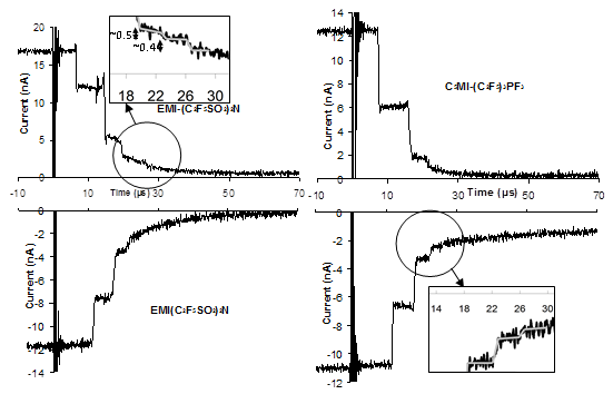
Time of flight mass spectra characteristic of the emissions from Taylor cones of two ionic liquids: right, C5MI-(C2F5)3PF3; left, EMI-(C2F5SO2)2N. The time traces result from deflecting the ion beam at time  and recording the decay of the collected current as a function of time. Top, positive electrospray; bottom, negative electrospray.
The Time of Flight Principle
Students will use the Time of Flight technique to measure the propulsive characteristics. As the ions are accelerated due to a potential f given by the needle to extractor potential difference, the potential energy is transformed into kinetic energy by the simple formula:
(5) 
By using a pulsing gate we can set an initial time for when the ions are allowed inside the chamber. Knowing the length L traveled by these ions, and reading the signal through an oscilloscope, one can calculate the total time for ions of a particular  ratio to reach the collector:
(6) 
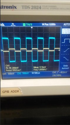
The Time of Flight will allow students to calculate the exhaust speed of the ions and from (1-4) the different propulsive characteristics of the ions. As an example of an ion beam captured by an oscilloscope, Figure 2 [8,21-22] shows raw data taken with an oscilloscope for very heavy Ionic Liquid species. The time can be read on the abscise in ms while the total current can be measured in nA. The different steps in the wave form correspond to the decay arrival of different species at the collector when the beam is deflected. These species are ions of the family [AB]nA+ or [AB]mB– depending on the polarity and n or m can be anywhere from 0-10. And A+ and B– correspond to the positive and negative ions.
-
Propulsive characteristics
Once raw spectra are collected, the students will proceed to de-convolute the data and apply electrical, mechanical and numerical knowledge to derive the propulsive characteristics of such liquids. For example, knowing the ToF of a fraction of particle current, , the mass flow rate can be written as:
(7) 
Similarly, the thrust can be calculated by multiplying the mass flow rate by the velocity:
(8) 
Integrating over the total time would yield the combined propulsive characteristics of the propellant. Figure 3 shows test candidate DMI-N(CN)2 in which flow rate, thrust, efficiency and specific impulse are calculated. Notably the Specific Impulse (without post acceleration) is already over 4000s. The downside is that the thrust per emitter is less than 1mN leading to the need of multiplexing (multiple emitters)[23].
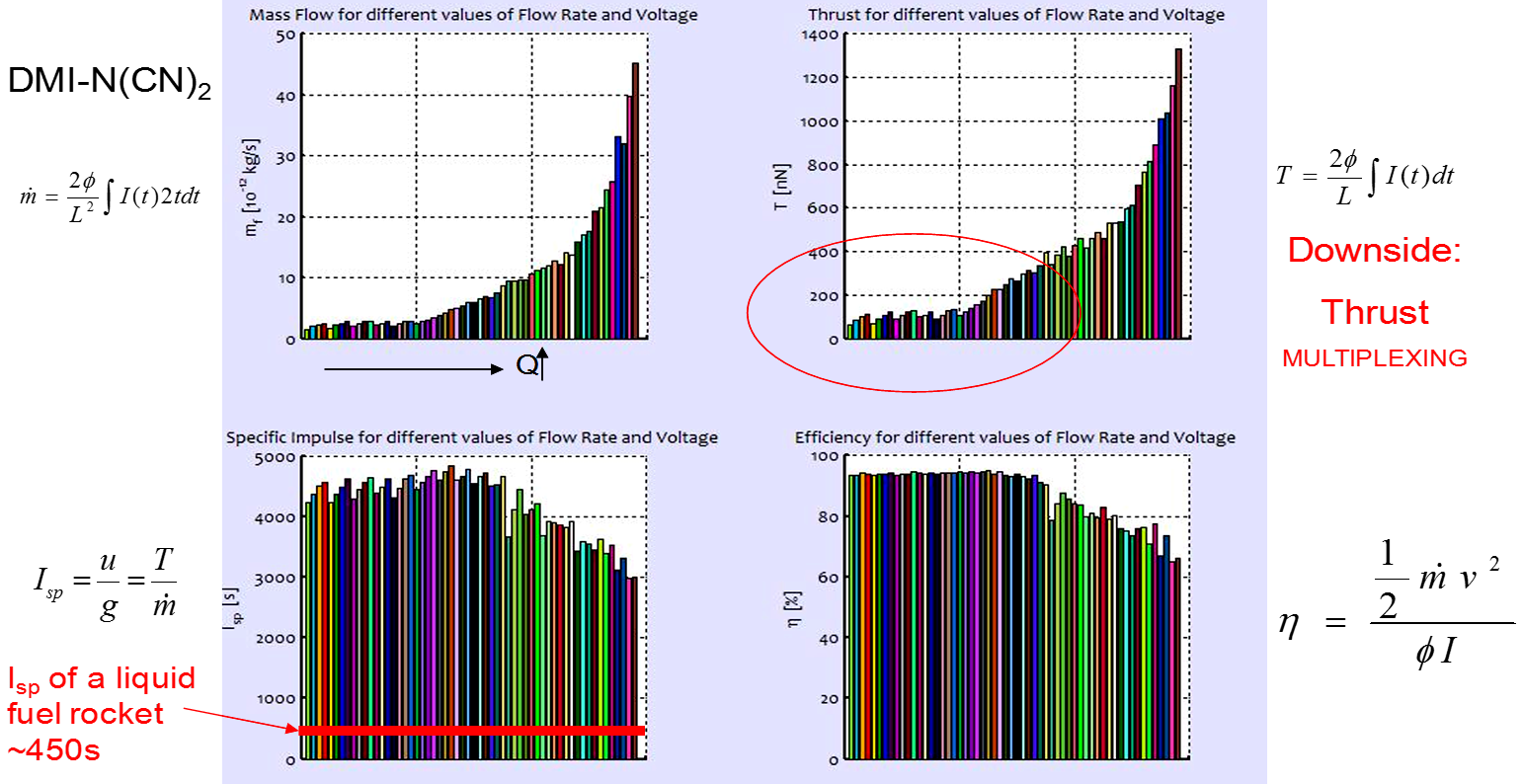
Mass Flow, thrust, specific impulse and efficiency (defined as: , where Isp is the specific impulse, T the thrust, g the gravity and I the current) for the ionic liquid DMI-N(CN)2 at f~2500V with no post acceleration.
MURI PROJECT
During the summer of 2016, Sajal Kherde, Bree Abernathy, Daniel Miller and Yanxiang Ding undertook the project of creating the first ever built Vacuum Time Of Flight Chamber in Mechanical Engineering at IUPUI in Indianapolis. This MURI project was made possible thanks partially to the Center for Research and Learning here at IUPUI.
In only 2 months, they were able to build the chamber from scratch, assemble an injector, collector and electrometer and test the results with multiple liquids. Here is their blog and results:
Week 1 (June 1st-5th 2016)
The first week was a very interesting week for the team. It began with the team meeting on Wednesday June 1st, followed by regular lab work. From the start, we knew that this project was not your regular undergrad project, but that we were here to do real research.
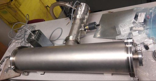
Time of Flight Chamber. Turbo and mechanical pump attached!
The chamber for the ToF had to be built from regular metal pieces that our advisors had already purchased. We got all the different dimensions needed to start the project. We inferred the correct dimensions of the collector plate, keeping in mind the angular spread of the electron beam and separation as a function of the distance. The rest of the chamber assembly, not including the injector piece, went smoothly without many hurdles. The only problem we ran into was with a missing connector part to connect the primary vacuum to the secondary one and had to be ordered.
By Thursday, the PCB boards for the dual stage electrometer/Operational Amplifier were designed and our primary vacuum was connected for testing purposes. We ran into a problem. Our mechanical pump ran at 220V and even though we had a transformer, its specifications were on the limit of the necessary power (220V/8A, 1.760kW) required for the mechanical pump to run and we constantly burnt the fuse.
Friday was a great day! We were able to connect the missing part and have a complete test run of the chamber and vacuums. The PCB was printed by evening and we were able to understand the working of the remote control to use with the turbo molecular pump. We were able to reach a low pressure of around 1.2E-07. We also were able to have the electrometer presentation prepared.
Week 2 (June 6th-12th 2016)
During the second week, the electrometer was built in order to measure electrical potential at extremely low values without drawing any current from the circuit. In order to make the electrometer, a layout was needed to be placed on a printed circuit board. We used Ultiboard to design the circuit diagram as shown below. The first stage of the electrometer has an amplification of 220k which is enough to convert nA of current into mV so that we could observe the signal in the oscilloscope. The second stage has an amplification of 10 and will only be used in cases where the signal was too small to be read by the oscilloscope.
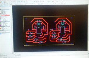
Two stage electrometer circuit design
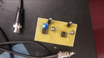
Circuit Board Printed. Let us add the components
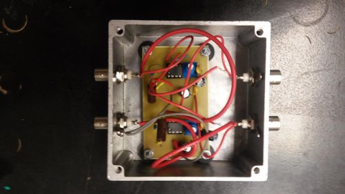
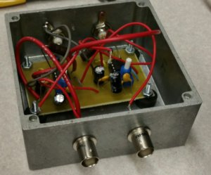
Electrometer assembled and put into the box. Ready to test it!
The circuit board was then printed out and the different parts were then soldered and assembled onto the board. Once done, we tested the gain using an oscilloscope. To test the results, we modified the gain of the first stage to be 10 so that we could use a mV square wave. The results were expected as the first stage of the electrometer had a gain of -10 and both stages together had a gain of 100. Once the desired results were obtained, the electrometer was then connected to the BNC connectors inside a Faraday cage. This Faraday cage is used to prevent the electrometer from seeing too much noise from the HV pulser. Note that the electrometer used uses a feedback loop on the negative side of the operational amplifier and therefore it is expected that the gain is inverted.
Bree is testing the electrometer and making sure that everything is properly working.
It works!!
Week 3 (June 13th-19th)
Mechanical
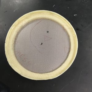
Collector finished
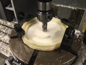
Collector isolation plastic being finalized in the mill
At the very beginning of week 3, we measured the dimensions of the chamber again to determine a more precise requirement for the collector plate. According to the requirements, i.e. that there should be enough gap between the plate and the chamber and that the mesh need to be ensured insulated to the chamber, we made some adjustment on the design of the collector plate. A 175 mm diameter metal plate was used to replace the original 190 mm diameter plate. The plastic plate was redesigned and processed to be suitable for the new metal plate. An ABS plastic edge was used to insulate the mesh and the chamber. After three days of learning, trying and overcoming different difficulties, we used the drilling machine and finished the manufacturing of the collector plate. The only thing missed for this part is a matching screw to fasten the metal plate, the plastic plate and the Teflon rod together. This will allow us to place the collector at any distance we wish from the injector.
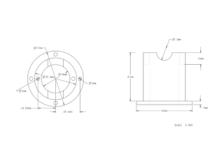
Creo 3D Model used to get accurate dimension to build the injector
Based on the requirements of the experiment, we redesigned the injector and re-determined the dimensions of the parts of it. As a high precision of process is desired, we used Creo to develop 3-D models of the injector so that a high quality manufacture is possible. Also, with great effort, we finally acquired the permission of using the CNC machine, which is under the charge of the Mechanical Engineering Technology department. It means that the components of the injectors can be processed with high efficiency and satisfactory quality. Hopefully, the injector will be finished in next week. By then, every major component of the experimental setup would be finished. And we can assemble them together and test the equipment. If everything goes smoothly, we are optimistic to get the experiments started in two weeks.
In addition, since the pulse generator, oscilloscope, function generator and the high voltage supply are already set up, we set up our work space for future experiment.
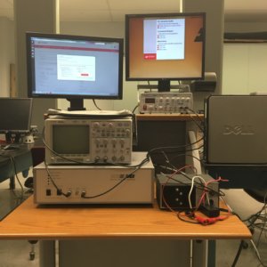
Experimental Setup
In a conclusion, we achieved satisfying progress in week 3. Things are getting ready for the fully commence of the experiment.
Electrical
Electrometer tested inside box
For week 3, the first iteration of the electrometer was successfully tested and completed: we used an oscilloscope to test the gain for each amplifier stage which led us to the discovery of a faulty operational-amplifier. After replacing the faulty op-amp with a new one and obtaining the desired gain, we added the 220KΩ resistor to the first stage, tested again, and confirmed the desired gain result. Next we finalized the electrometer by trimming excess wire on the board’s underside and drilling 4 holes (one per corner) in which to screw on small rubber “feet” so that the board may stand evenly and securely inside the metal housing apparatus.
![\[\]](https://www.imospedia.com/wp-content/ql-cache/quicklatex.com-5a8454e4168ec940c5c7f5eac46402a2_l3.png "Rendered by QuickLaTeX.com")
Next we hooked up our oscilloscope and computer for data acquisition and analysis: our particular oscilloscope/software requires an RS-232-C connection. We had a DB9 Serial RS-232 cable with two male ends, but our PC port was also male (see images below for detail) so we obtained the proper adapter and hooked it up accordingly.
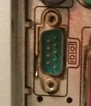
RS-232 Male Port on PC
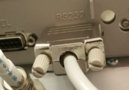
RS-232 connection to Oscilloscope

Both RS-232 were male
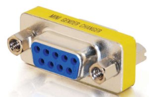
The adapter we purchased
Lastly, we designed another circuit using MOSFET transistors to work as an alternative switch to implement our high-voltage gate. Below are the circuit diagram and the schematic created for the circuit board using Ultiboard software.
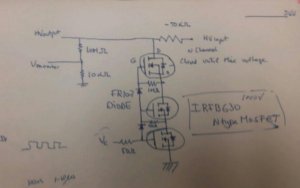
HV Switch using MOSFETS
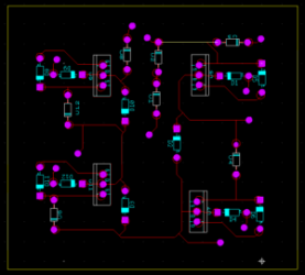
Switch Schematic. Ready to print
For the coming week (week 4) we will continue building and begin subsequent testing of this circuit, as well as begin coding for data acquisition / analysis.
Week 4 (June 20th-26th)
Electrical
This week we built 2 power supply boxes that each contained an AC-DC power module, an AC wall outlet, a switch, an LED (to signify switch “ON”) and outputs. One box provides the required +15V / -15V to the electrometer and the other box provides the required -15V to the collector. The images below show a box under construction, and the two completed boxes together:
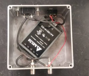
Power supply for Electrometer.
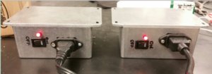
Two power supplies are ready
After constructing the boxes, we hooked up the electrometer’s box to verify that everything is working correctly, and indeed everything worked as expected. We will test the other box for the collector when the collector is ready. Below is an image of the electrometer outputting the desired waveform when tested with its power supply box:
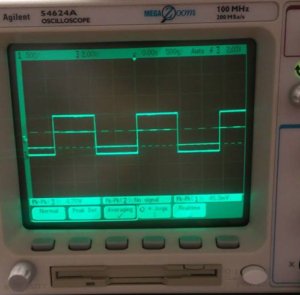
Oscilloscope reading signal from Electrometer
We also built another box for the High Voltage (HV) power supply (see image below, bottom right) which houses all of the live and grounding wires that connect the HV supply to other including the high voltage pulsar and the DC power supply.
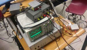
Oscilloscope, electrometer setup
The circuit board of the HV supply we’re building with transistors was also redesigned (see image below) to improve reliability and ease of use as the original had the potential to create a short and had unnecessary components.
Switch diagram redesigned
Week 5 (June 27th-July 3rd)
Mechanical
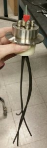
These two weeks have been very productive. We have got the entire chamber ready.We finalized emitter done. It did take us through several challenges and we wereable to overcome them with success.
The chamber had to be screwed properly, the main screw caused a bit of trouble as it was too tallcausing a problem as is located at the center, where the main beam is thought to hit. So we filed it downto a short height preventing any intrusion. Also, the wiring method was to be finalized as we hadproblems soldering the copper BNC wires to the mesh as well as the collector plate. For the collectorplate, we made sure the wire is sandwiched properly between the plastic casing and the metallic plate,ensuring proper contact. For the mesh, we decided to insert a small metallic ring on one side and thecopper wire, which passed through one of the holes in the mesh, allowing us to use the sandwichmethod once again to ensure a working connection. The wires were then epoxied to to the plastic on theback to ensure a tight fitting and secure connection.
The emitter casing had to have a few holes made to allow for the wires from the outer most connectorto be connected to the meshes in the emitter chain, and for three screws to be threaded in to allow us tocenter the needle casing.
The main chamber was altered this week to reduce the distance between the first mesh and the beamconstrictor. We had to have the original chamber cover cut off and then welded once again to view portchamber. We ran into a problem when we detected a minor leak and had it fixed using varioustechniques.
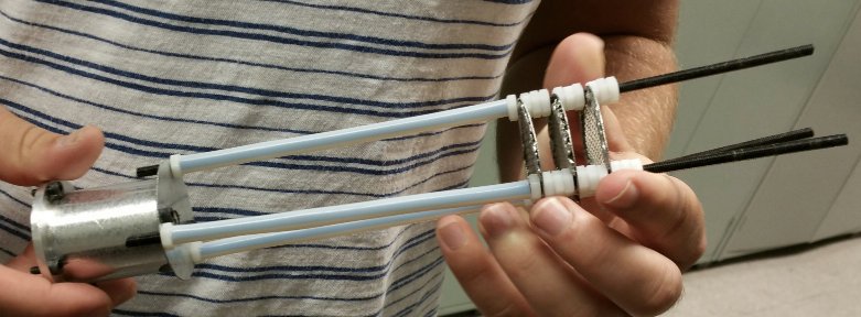
The meshes were lined up on nylon rods, distanced by nylon nuts and connected to the outermostemitter part. The distance had to be altered few times but in the ended we achieved success in itsconstruction. The meshes were also wired this week allowing us to begin testing in the beginning of thefollowing week.
Electrical
Week 5 was an exciting week—we are close to finishing building and hope to begin testing by the end of next week! Highlights of week 5 include:
 The transistors for our pulsar circuit arrived, but we are still waiting for the PCB to be created so that we can build that circuit.
- We worked with CNC to get the necessary software for our oscilloscope installed on our lab PC, and have used it to successfully interface with the oscilloscope.
- We discovered the BNC cable heads going into the electrometer stuck out too far off the collector plate to fit inside the chamber, so we attached BNC T-connectors to the electrometer’s BNC ports. This allowed us to rotate the heads parallel to the electrometer instead of perpendicular.
- We discovered and fixed a pressure leak in the chamber.
- We soldered the electrometer’s input wire to collector plate and soldered the -15V power supply wire to the collector mesh.
- We connected the cables for electrometer and both power supply boxes and assembled the back of the chamber. We also soldered the 4 high-voltage wires to their respective connections on the inside of the injector.
- We applied some finishing touches (e.g. re-soldering and filing edges) to the 3 meshes comprising the Gate and assembled them onto the 3 nylon rod
For next week, we plan to finish building the chamber in order to connect all cables and equipment so that we can begin testing! We will also be meeting with Dr. Izadian to learn how we may be able to use a DSpace controller and Simulink software for data acquisition and analysis.
Week 6-9 (July 3rd-August 1st)
During the final three weeks of the MURI project, we started doing experiments. This is what the complete setup looks finally:
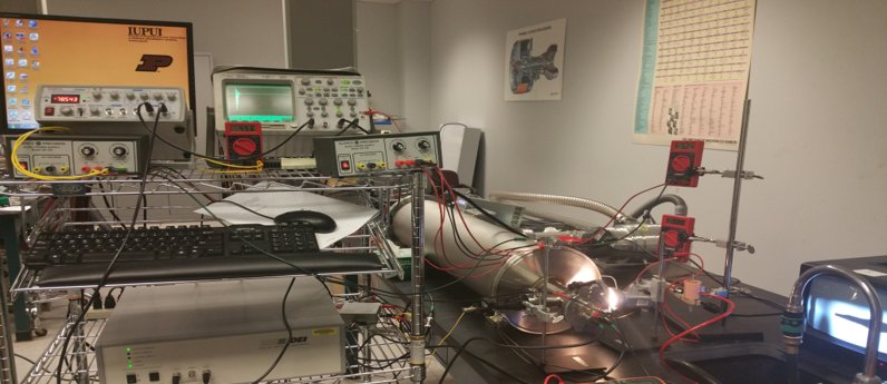
Complete Setup. We are ready to start experiments and gather data!!
The silica capillary, which lies inside the chamber under vacuum, can be observed on a screen to the right.
The Data gathered throughout the weeks was analyzed and put together in a poster which can be downloaded for anyone to check:

This is us presenting our poster at the Center for Research and Learning Poster Symposium on July 28th 2016. Cheers!!

From Left to Right: Daniel Miller, Yanxiang Ding, Bree Abernathy, Sajal Kherde
REFERENCES
[1] Lozano P.. Studies on the Ion-Droplet Mixed Regime in Colloid Thrusters. PhD thesis, Department of Aeronautics and Astronautics, M.I.T., 2003.[2] Fernandez Garcia, J.. Characterization of new Ionic Liquids for their application in Electrospray-based Space Propulsion. Thesis Yale 2008.
[3] Jahn, R.G., Choueiri. E.Y. Electric Propulsion. In Encyclopedia of Physical Science and Technology, volume 5. Academic Press, third edition, 2002.
[4] Garoz, D., Bueno, C., Larriba, C., Castro, S., Romero-Sanz, I., de la Mora, J. Fernández, Yoshida, Y., Saito, G. (2007). “Taylor cones of ionic liquids from capillary tubes as sources of pure ions: The role of surface tension and electrical conductivity.” Journal of Applied Physics 102(6): 064913-1-10.
[5] Loscertales, I. G. and F. De la mora, J. (1995). “Experiments on the Kinetics of Field Evaporation of Small Ions from Droplets.” Journal of Chemical Physics 103(12): 5041-5060.
[6] Romero-Sanz I, Bocanegra R., Fernández de la Mora J., and Gamero-Castaño M. 2003. Source of heavy molecular ions based on Taylor cones of ionic liquids operating in the pure ion evaporation regime, Journal of Applied Physics. 94:3599-05
[7] Lozano, P. and Martinez-Sanchez M. (2005). “Ionic liquid ion sources: Characterization of externally wetted emitters.” Journal of Colloid and Interface Science 282(2): 415-421.
[8] Larriba, C., Castro, S. et al. (2007). “Monoenergetic source of kilodalton ions from Taylor cones of ionic liquids.” Journal of Applied Physics 101(8): 1-6.
[9] Dole, M., Mack, L. L. , et al. (1968). “Molecular Beams of Macroions.” Journal of Chemical Physics 49(5): 2240-.
[10] Iribarne, J. V., Thomson, B. A. (1976). “Evaporation of Small Ions from Charged Droplets.” Journal of Chemical Physics 64(6): 2287-2294.
[11] Martino, W., F. de la Mora, J., et al. (2006). “Surface tension measurements of highly conducting ionic liquids.” Green Chemistry 8(4): 390-397.
[12] Yoshida, Y., Baba O., Larriba C., (2007). “Imidazolium-based ionic liquids formed with dicyanamide anion: Influence of cationic structure on ionic conductivity.” Journal of Physical Chemistry B 111(42): 12204-12210.
[13] Larriba, C. et al. “Ionic Liquids IV”, not just solvents anymore, ISBN: 9780841274457 (Book) ACS chapter 21.
[14] J. O’M Bockris, A. K. N. Reddy, Modern Electrochemistry 1 ISBN 0-306-45554-4, Chapter V, 632-645.
[15] Fürth, R. (1941). “On the stability of crystal lattices VI. The properties of matter under high pressure and the lattice theory of crystals.” Proceedings of the Cambridge Philosophical Society 37: 177-185
[16] Fürth, R. (1941). “On the theory of the liquid state I. The statistical treatment of the thermodynamics of liquids by the theory of holes.” Proceedings of the Cambridge Philosophical Society 37: 252-275.
[17] Larriba, C., Yoshida, Y. et al. (2008). “Correlation between surface tension and void fraction in ionic liquids.” Journal of Physical Chemistry B 112(39): 12401-12407.
[18] Saville, D. A. (1997). “Electrohydrodynamics: The Taylor-Melcher leaky dielectric model.” Annual Review of Fluid Mechanics 29: 27-64.
[19] Bailey, A. G. (1988) “Electrostatic Spraying of Liquids”, Wiley, New York.
[20] Fenn, J. B., Mann, M., Meng, C. K., Wong, S. F., Whitehouse, C. M. (1989). “Electrospray Ionization for Mass-Spectrometry of Large Biomolecules.” Science 246(4926): 64-71.
[21] Zeleny, J. (1914). “The electrical discharge from liquid points, and a hydrostatic method of measuring the electric intensity at their surfaces.” Physical Review 3(2): 69-91.
[22] Taylor, G. (1964). “Disintegration of Water Drops in Electric Field.” Proceedings of the Royal Society of London Series a-Mathematical and Physical Sciences 280(138): 383-.
[23] Cloupeau, M. and B. Prunetfoch (1989). “Electrostatic Spraying of Liquids in Cone-Jet Mode.” Journal of Electrostatics 22(2): 135-159.
[24] Cloupeau, M. and B. Prunetfoch (1990). “Electrostatic Spraying of Liquids – Main Functioning Modes.” Journal of Electrostatics 25(2): 165-184.
[25] Gamero-Castano, M. and J. F. de la Mora (2000). “Direct measurement of ion evaporation kinetics from electrified liquid surfaces.” Journal of Chemical Physics 113(2): 815-832.
[26] Iribarne, J. V. and B. A. Thomson (1976). “Evaporation of Small Ions from Charged Droplets.” Journal of Chemical Physics 64(6): 2287-2294.
[27] Castro, S., Larriba, C. et al. (2007). “Effect of liquid properties on electrosprays from externally wetted ionic liquid ion sources.” Journal of Applied Physics 102(9):1 -6.
[28] Castro, S. and F. de la Mora, J. (2009). “Effect of tip curvature on ionic emissions from Taylor cones of ionic liquids from externally wetted tungsten tips.” Journal of Applied Physics 105(3): -.
[29] Deng, W. W., J. F. Klemic, et al. (2006). “Increase of electrospray throughput using multiplexed microfabricated sources for the scalable generation of monodisperse droplets.” Journal of Aerosol Science 37(6): 696-714.
