Hello, I’m Xi Chen, a PhD student of Mechanical Engineering in Purdue University. I’m studying in Dr. Carlos’s group and my research area is to develop new instruments for Aerosol research. Here, I’m so happy to have the chance to learn the knowledge about how to separate the particles with different mobilities and got familiar with the current instruments used for the researches. Besides, after communicating with other scholars, I had a deep understanding of the aerosol potential use in a wide range of areas, like chemistry, physics, biology and environment.

To overcome the shortages for current instruments, Dr. Carlos introduced a new model-Inverted Drift Tube (IDT). The IDT consists of two varying force: Electrical field, which proportional to axis distance but in negative direction; the other one is drag force, which is in positive direction, as shown in Figure 1.

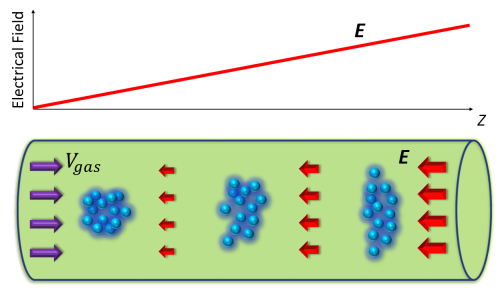
Figure 1. Model of Inverted Drift Tube

IDT applied the Intermittent Push Flow method and has an advantage of diffusional auto correction, which will produce a higher resolution compared with regular drift tube. Since theoretical study and numerical simulation had been tested yielding promising results, my current work is to get the high resolution results from experiment.

Besides, Dr. Carlos gave me the chance to learn how to build up a model (by Solidworks, Figure 2), simulate the fluid flow (by Ansys-Fluent, Figure 3), and also simulate the particles flying through the drift tube (by Simion, Figure 4).

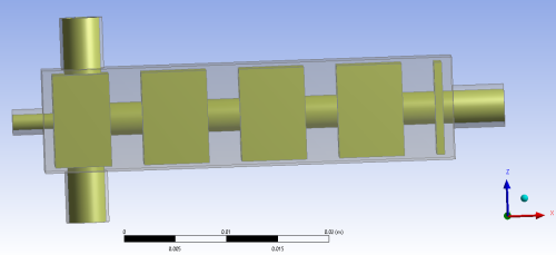
Figure 2. A new designed model for separating charged and uncharged particles. The yellow part means the fluid domain, and the transparent part means the solid domain.

Figure 2 shows the model generated by Solidworks. The model consists of a square cavity with 2 inlets (in x direction) and 2 outlets (in z direction) and 4 square electrodes with a circular hole in the middle of it. This model would be reloaded into Ansys-Fluent to get the velocity field in the fluid domain.

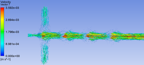
Figure 3. Ansys-Fluent simulation results for the velocity vector.

Figure 3 shows the velocity field in the fluid domain. The velocity profile would be interpolated and then be applied into Simion to give a velocity field and it would simulate the trajectories of the mobilities.

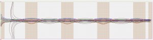
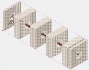
Figure 4 (a-b). Simion simulation of the trajectories of particles with different mobilities. (a) x-z plane version. The black lines show the trajectories of uncharged particles, and the others of different colors represent different mobilities. It’s obvious that the uncharged particles will get seperated with the charged particles. (b)The 3-D version of trajectories.

I have learned a lot and during these process, and enjoyed the working environment in the lab. Thanks to Dr. Carlos and my teammates, they gave me too much help about the experiment, and the most important thing is that, I found the method to study and improve myself.